
Motion Control Precision: Servo Loops, Fieldbus Jitter, AI
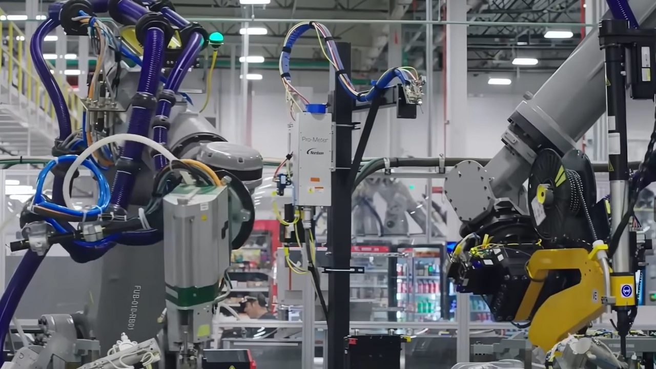
TL;DR: Motion control precision is set by a hierarchy of loops running at very different speeds, not by a single “AI-ready” controller. On a high-performance servo axis the current loop closes every 62.5 to 125 µs, position setpoints typically cross the fieldbus every 250 µs to 1 ms, and the synchronisation jitter of that bus is held to about 1 µs. Cameras deliver a new frame every 8 to 33 ms, wrist force/torque sensors update at 1 to 7 kHz, and learned visuomotor policies still issue commands at roughly 10 Hz. “Perception-decision-execution integration” describes an architecture, not a shipped capability: the deterministic layers are mature and measurable, while AI sits above them, converting perception into waypoints that classical servo loops execute.
What actually determines motion control precision?
Motion control precision is the sum of four independently measurable error sources: feedback resolution, control-loop bandwidth and update rate, time synchronisation between axes, and mechanical compliance between the motor and the tool. A faster processor does not fix a compliant mechanics stack, and a higher-resolution encoder does not fix a 10 ms network jitter problem. Precision improves only when the weakest term in that budget improves.
The error budget is worth writing down before comparing architectures. Position error at the tool comes from encoder quantisation and interpolation, following error while moving, the phase lag introduced by sampling and filtering, axis-to-axis skew from unsynchronised clocks, and deflection in couplings, gearboxes and frames. On a machine that moves at 200 mm/s, a 100 µs timing error displaces the tool by 20 µm; a 1 µs error displaces it by 0.2 µm. That arithmetic is why fieldbus synchronisation specifications are quoted in microseconds while camera specifications are quoted in frames per second.
Following error is equally mechanical in its behaviour. In a purely proportional position loop, the steady-state following error is approximately the feed rate divided by the position-loop gain, so a machine running at 100 mm/s with a 30 s-1 gain lags by several millimetres before velocity feedforward is applied. Feedforward, higher loop rates and stiffer mechanics reduce that lag, but none of them removes it. Any claim about “real-time execution” has to be read against this budget rather than in isolation.
How fast do servo current and velocity loops actually run?
Published high-performance servo drives close the current loop every 62.5 to 125 µs, equivalent to 8 to 16 kHz, and the velocity loop every 16 to 125 µs depending on the design. These are vendor-specific figures from product documentation, not an industry-wide minimum, and mid-range drives often run the same loops at half those rates.
Beckhoff specifies a shortest current-controller cycle of 62.5 µs at an 8 kHz switching frequency for the AX8000, with the current controller reacting to setpoint deviations within 1 µs and the velocity controller cycling at about 16 µs at a 32 kHz switching frequency. Siemens specifies a 62.5 µs current-controller cycle for the SINAMICS S210, and 125 µs for the PROFINET variant of the S200 family. Mitsubishi quotes a 62.5 µs minimum operation cycle for four-axis control on its MR-EM441G embedded motion board. Those three figures come from three different architectures and should not be generalised to every drive on a machine.
Bandwidth is a separate specification and is frequently confused with update rate. Yaskawa quotes a 3.1 kHz speed-loop frequency response for the Sigma-7 series with a 24-bit encoder; that number describes how the loop responds to a sinusoidal speed command, not how often it executes. A drive can advertise a high response frequency while its current loop runs at 8 kHz, and a machine builder comparing datasheets needs to check both numbers plus the filter settings that were active during the measurement.
Position control is usually closed one level up, in the motion controller or CNC, at 0.5 to 4 ms. The drive receives a new position setpoint each cycle and performs fine interpolation between setpoints, so the motor current is updated thousands of times per second while the commanded path is recalculated hundreds of times per second. In retrofit work this split matters: a replacement amplifier such as a Mitsubishi MELSERVO-J3 servo drive with SSCNET III/H or a Lenze ECS 16 A servo drive module has to match the host controller’s cycle and interpolation behaviour, not just its power rating.
What do EtherCAT and PROFINET IRT cycle times actually guarantee?
EtherCAT is designed around cycle times of 100 µs or less with jitter of 1 µs or less, using distributed clocks for synchronisation; multi-axis servo systems commonly run at 100 to 250 µs. PROFINET IRT (Conformance Class C) defaults to a 250 µs update and can reach 31.25 µs, with jitter of about 1 µs; Conformance Class D moves the same mechanisms onto TSN.
The EtherCAT Technology Group states that short cycle times (≤ 100 µs) and low jitter (≤ 1 µs) were the design focus of the protocol, which is specified in IEC 61158. A Beckhoff XFC demonstration ran a control cycle of 12.5 µs with 15 slaves, which shows the floor of the technology rather than what a typical machine needs. Integrator guidance for multi-axis servo systems puts practical cycle times at 100 to 250 µs, with longer cycles acceptable when position control is closed in the drive.
For PROFINET, the system description sets the minimum update rate for Conformance Class C at 250 µs by default, reducible to 31.25 µs depending on hardware, and the PROFINET System Description sets the Conformance Class C minimum at 31.25 µs, and PI’s own FAQ describes IRT jitter as below 1 µs. An important architectural difference is that PROFINET IRT reserves bandwidth through scheduled switching, while EtherCAT processes frames on the fly in each slave. Both achieve deterministic behaviour; they achieve it differently, and a machine’s existing network topology usually decides which one is available.
The guarantee is narrower than marketing language suggests. The bus cycle determines how often setpoints and actual values cross the network. It does not determine the drive’s internal current-loop rate, and it does not by itself synchronise the mechanical outcome across axes. That requires a common time base: distributed clocks in EtherCAT, and time synchronisation derived from IEEE 1588 / IEEE 802.1AS in the PROFINET case. Products such as a 32-axis EtherCAT CPU module or a 16-axis EtherCAT motion controller expose those settings directly, and a Lenze PROFINET RT communication module shows the other side of the same decision for a drive-based architecture.
Why does jitter matter more than average latency?
Average latency shifts a trajectory in time and can be compensated by look-ahead; jitter changes the spacing between samples and cannot. A 1 µs synchronisation error at 1 m/s produces a 1 µm position error, while a 100 µs jitter spike at 200 mm/s produces 20 µm, which is larger than the repeatability of many machine tools.
This is the practical reason distributed clocks exist. In a multi-axis interpolation, all axes must apply their setpoints at the same instant. If one axis receives its setpoint 50 µs late, the tool deviates from the programmed path even though every axis tracked its own command perfectly. EtherCAT aligns slave clocks to a reference clock, and PROFINET IRT distributes a common cycle counter; both are designed so that the residual skew stays near 1 µm at typical feed rates.
Jitter also enters through the operating system. A general-purpose or even a PREEMPT_RT Linux kernel running perception, logging or GPU work on the same cores as the motion task can produce scheduling spikes in the tens to hundreds of microseconds; one published integrator benchmark on an embedded GPU module reported spikes above 100 µs under combined GPU, storage and EtherCAT load until CPU isolation was applied. The safe pattern is architectural: keep the hard real-time loop on a dedicated core or in the drive, and keep the non-deterministic workload elsewhere.
How fast can vision, force and position sensors feed the loop?
Position feedback is the fastest sensor in the chain: EnDat 2.2 transfers absolute position at clock rates up to 16 MHz, and 24-bit single-turn encoders are standard on servo motors. Wrist force/torque sensors update at roughly 1 to 7 kHz, while industrial cameras deliver 30 to 120 frames per second, with 120 to 200+ fps reserved for high-speed pick-and-place. The gap between the fastest and slowest sensor is about three orders of magnitude.
Heidenhain specifies EnDat 2.2 clock frequencies up to 16 MHz with propagation-delay compensation, and up to 100 m of cable at 8 MHz. That is the channel that makes a 62.5 µs current loop meaningful: without a position update of comparable freshness, the loop is regulating against stale data. Encoder mounting hardware belongs in the same discussion, because a 10 mm bore encoder coupling that slips or winds up adds mechanical error after the encoder has measured it.
Force and torque sensing sits in the middle of the range. Six-axis sensors are specified for maximum update rates around 7 kHz, and contact-rich assembly research commonly logs or controls at 500 Hz to 1 kHz. That is fast enough for impedance and force control, and roughly one to two orders of magnitude slower than the current loop. Vision is slower again: at 30 fps a new frame arrives every 33 ms, and even at 120 fps the interval is 8.3 ms. A camera therefore cannot close a position loop in the sense a servo drive does. It can update a target, correct a calibration drift, or verify a placement.
Where the measurement is a distance rather than an image, the numbers improve but stay in the millisecond domain. A high-speed laser distance sensor rated for 15 m/s is specified for moving-target measurement, and an analog laser distance sensor provides a continuous position signal for slower axes. Neither replaces the motor encoder, and both are subject to their own response time, which must be added to the error budget rather than assumed away.
Where does edge AI inference fit in the control chain?
Edge inference fits above the servo loop, not inside it. Perception networks on embedded GPU modules typically take single-digit to tens of milliseconds per frame; learned manipulation policies issue action chunks at around 10 Hz; large language or vision-language models can take seconds per inference. None of those latencies is compatible with a 62.5 µs current loop, which is why production architectures keep the AI layer asynchronous and let classical control interpolate its output.
A concrete published example shows the pattern. Diffusion Policy, a widely cited visuomotor policy, predicts robot commands at 10 Hz and those commands are then linearly interpolated to 125 Hz for execution on a UR5. The learned model decides where to go; the robot controller decides how to get there at millisecond resolution. NVIDIA’s Holoscan robotics stack demonstrates the same split from the other direction, running a gravity-compensation loop at 400 Hz from joint state while perception and GPU work run on separate execution paths.
The latency of larger models sets the boundary. NVIDIA’s published Jetson benchmarks list single-stream latency of about 10.2 seconds for GPT-J 6B on AGX Orin, which is not a control model but illustrates the order of magnitude involved when a large network is placed on an embedded module. Inference latency is also variable, because it depends on batch size, thermal state and memory bandwidth. A control architecture that assumes a fixed inference time will fail intermittently, which is exactly the failure mode that deterministic fieldbuses were invented to eliminate.
The reasonable division of labour is therefore hierarchical. Task planning and perception run at 1 to 50 Hz, trajectory generation at 10 to 100 Hz, interpolation and position control at 250 Hz to 2 kHz, and current control at 8 to 16 kHz. “Perception-decision-execution integration” is a description of how those layers exchange data, not evidence that they have collapsed into one loop.
How do the three motion control architectures compare?
The generational comparison is often presented as a replacement story. In engineering terms it is a change in where the target comes from and at what rate it can be updated, while the execution layer stays largely the same.
| Architecture | Where the target comes from | Typical decision rate | What sets the error floor | Timing requirement | Production status |
|---|---|---|---|---|---|
| Pre-programmed trajectory | CAM or motion controller, fixed path | 0.5–4 ms position updates; 62.5–125 µs current loop | Encoder resolution, following error, mechanical compliance | Hard real-time, ≈1 µs axis synchronisation | Mature, dominant in production |
| Visual servoing | Camera-derived pose or feature error | 30–120 fps; 8–33 ms per update | Calibration, image resolution, vision-to-motion latency | Soft real-time; latency compensation required | Mature for stop-and-go and slow tracking; limited at high speed |
| Learning-based control | Learned policy from images, force and proprioception | Around 10–50 Hz action chunks, interpolated upward | Policy generalisation, data coverage, inference latency | Best-effort; must be wrapped by a deterministic loop | Pilot and limited production, usually above classical control |
The table explains why “real-time AI control” claims need qualification. A visual servo loop at 30 fps has a 33 ms sampling interval, which limits its usable closed-loop bandwidth to a few hertz; a learned policy at 10 Hz is slower still. Both can achieve impressive task-level accuracy when the underlying servo layer holds position precisely between decisions. Neither can substitute for that layer when the requirement is sub-millimetre tracking at speed.
Which parts of the integrated architecture are already shipped?
The deterministic layers are shipped and measurable: current, velocity and position loops in the drive, distributed-clock synchronisation, absolute encoder interfaces, and force-controlled assembly at 1 kHz. The AI layers are shipped as perception modules and policy generators that run above those loops. End-to-end learned control of a servo axis, and inference inside the current loop, remain experimental or vendor-specific demonstrations.
Mature, in volume production: servo drives with published current-loop rates; EtherCAT and PROFINET IRT networks with microsecond synchronisation; 24-bit absolute encoders; force/torque-controlled insertion and pressing; vision-guided pick-and-place where the robot stops or slows to acquire the target. These are specified in datasheets and can be verified on a machine.
In pilot or limited deployment: continuous high-speed visual servoing on fast-moving conveyors; learned policies for contact-rich assembly, usually generating waypoints or impedance parameters rather than motor currents; on-drive analytics and anomaly detection; AI-assisted tuning that proposes gain sets for an engineer to accept. These exist in production at individual sites, but the published evidence is usually task-specific rather than a general capability.
Not generally available: a learned controller closing a current loop at 8 to 16 kHz on a standard industrial drive; a vision-language-action model issuing motor commands directly without an interpolation layer; any architecture that removes the deterministic fieldbus from a multi-axis machine. Those remain research directions, and the timing arithmetic above explains why.
How should precision be specified for a real machine?
Start from the required tool accuracy, then work backwards. Convert it into an allowed encoder resolution, an allowed following error at the maximum feed rate, an allowed axis skew, and an allowed mechanical deflection. Compare those allowances with the products on the machine: the drive’s current-loop rate, the controller’s position-loop rate, the bus cycle and jitter, the encoder interface and the coupling stiffness. A B&R 8LSA synchronous servo motor and a Lenze 9400 motion control module may both be correct choices for a retrofit, but only one combination will meet a 20 µm contour tolerance at the programmed feed rate.
Two practical checks catch most specification errors. First, confirm that the position-loop rate is at least ten times the highest frequency content in the trajectory; a 4 ms loop cannot faithfully execute a path with significant content above 25 Hz. Second, confirm that the synchronisation specification is quoted for the same network load as the application, because jitter figures measured on an idle network are not transferable to a network carrying drive, I/O and safety traffic. Where the machine already runs a known ecosystem, related builds such as the Omron C6 servo platform or a CompactLogix 5390 controller rated for 128 axes illustrate how loop rates and axis counts are traded in practice.
Sources and standards
- EtherCAT Technology Group: technology overview — design focus on cycle times ≤ 100 µs and jitter ≤ 1 µs, IEC 61158 reference, distributed clocks.
- Beckhoff AX8000 multi-axis servo system — 62.5 µs current-controller cycle at 8 kHz, velocity controller around 16 µs at 32 kHz, 1 µs reaction to current deviation.
- Beckhoff press release: new setpoint values every 62.5 µs — vendor comparison against 1 ms control systems.
- Siemens: SINAMICS S210 motion control — 62.5 µs current controller and 250 µs PROFINET IRT.
- Siemens: SINAMICS S200 overview — 125 µs current controller on the PROFINET variant, 62.5 µs on other variants.
- PROFINET System Description — Conformance Class C default 250 µs, minimum 31.25 µs.
- PROFINET community FAQ — conformance classes, IRT jitter below 1 µs, CC-D for TSN.
- Yaskawa Sigma-7 series — 3.1 kHz speed-loop frequency response, 24-bit encoder.
- Mitsubishi Electric MR-EM441G — 62.5 µs four-axis control cycle.
- Heidenhain: EnDat 2.2 interface — clock frequencies to 16 MHz, cable length limits with propagation-delay compensation.
- Diffusion Policy: visuomotor policy learning — commands predicted at 10 Hz and interpolated to 125 Hz for execution.
- NVIDIA: robot arm control with Holoscan — 400 Hz joint-state loop alongside GPU perception.
- NVIDIA Jetson benchmarks — single-stream latency figures for large models on embedded modules.
What is a typical servo current loop update rate?
High-performance industrial drives publish current-controller cycles of 62.5 to 125 µs, equivalent to 8 to 16 kHz. Beckhoff specifies 62.5 µs for the AX8000 at 8 kHz switching, Siemens specifies 62.5 µs for the SINAMICS S210 and 125 µs for the PROFINET variant of the S200, and Mitsubishi quotes a 62.5 µs four-axis cycle for the MR-EM441G. Mid-range drives commonly run at half those rates, so the figure has to be read from the specific product documentation rather than assumed for a whole machine.
What is the minimum EtherCAT cycle time for motion control?
EtherCAT was designed around cycle times of 100 µs or less, and the EtherCAT Technology Group’s XFC demonstration reached 12.5 µs with 15 slaves. Real multi-axis servo systems usually run at 100 to 250 µs. The cycle time is not the same as the drive’s current-loop rate: the bus determines how often setpoints cross the network, while the drive continues to regulate current between frames.
Is PROFINET IRT fast enough for servo control?
Yes. Conformance Class C defaults to a 250 µs update and can reach 31.25 µs on suitable hardware, with jitter of about 1 µs. Conformance Class D adds TSN mechanisms for the same purpose. Whether IRT is available depends on the controller, the switches and the drive’s interface, which is why retrofit projects often inherit the network type already installed rather than choosing freely.
Does a higher camera frame rate improve motion control accuracy?
Not directly. A 30 fps camera produces a new measurement every 33 ms, and 120 fps gives 8.3 ms; both are far slower than the servo loop. Frame rate improves the freshness of a vision-derived target, but the achievable accuracy still depends on calibration, image resolution, exposure time and the latency of the vision pipeline. High-rate visual servoing is viable for slower processes and is usually combined with the drive’s own encoder loop for fast motion.
Can AI inference run inside a 1 kHz servo loop?
Not for general-purpose models. Perception networks typically need single-digit to tens of milliseconds per inference, learned manipulation policies issue commands at around 10 Hz, and large models on embedded modules take hundreds of milliseconds or more. Production architectures therefore run inference asynchronously and let the motion controller or drive interpolate and execute the result at kilohertz rates.
What limits trajectory accuracy most: the drive, the bus or the mechanics?
Whichever term is largest in the error budget. A drive with a 62.5 µs current loop cannot compensate for a coupling that winds up, and a bus with 1 µs jitter cannot compensate for a 10 ms position-loop update. In practice, following error at feed rate, encoder resolution, axis synchronisation and structural compliance each contribute, and improving the weakest one produces the visible gain.